Comparing ADF Test Functions in R
In one of my last posts I was not sure how R’s different ADF test functions worked in detail. So, based on this discussion thread I set up a simple test. I created four time series:
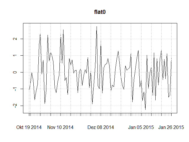
- flat0: stationary with mean 0,
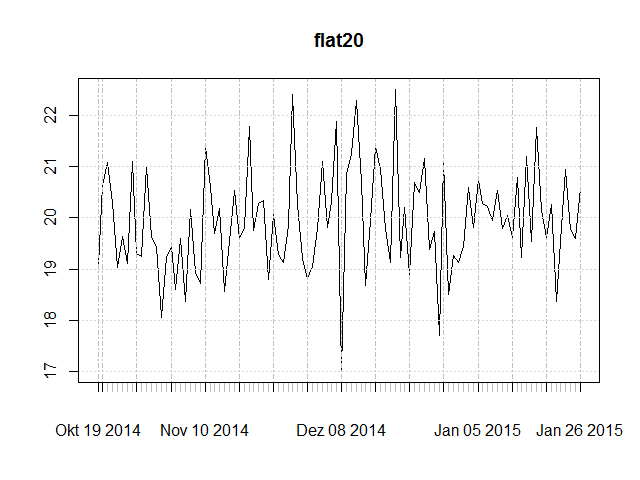
- flat20: stationary with mean 20,
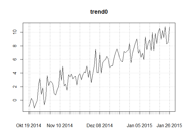
- trend0: trend stationary with “trend mean” crossing through (0, 0) - i.e. without intercept,
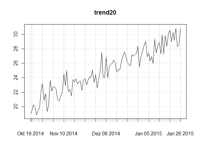
- trend20: trend stationary with “trend mean” crossing through (0, 20) - i.e. with intercept 20.
library(tseries)
library(xts)
library(fUnitRoots)

flat0 <- xts(rnorm(100), Sys.Date()-100:1)
plot(flat0)

flat20 <- xts(rnorm(100), Sys.Date()-100:1)+20
plot(flat20)

trend0 <- flat0+(row(flat0)*0.1)
plot(trend0)

trend20 <- flat0+(row(flat0)*0.1)+20
plot(trend20)
Here are corresponding plots:
 Notice the mean at the zero line and the absence of a trend.
 Notice the mean at the 20 line and the absence of a trend.
 Notice that the trending mean crosses the origin (0, 0) and the presence of a trend with slope 0.1.
 Notice that the trending mean crosses the (0, 20) point and the presence of a trend with slope 0.1.
Next, I calculated ADF tests using both the adf.test function in the tseries package and the adfTest function in the fUnitRoots package. We must keep in mind the following few points:
adf.testin tseries always automatically detrends the given time series.adfTestin fUnitRoots has three different type options:nc,candct.
From R’s documentation of the adfTest function:
_type_: a character string describing the type of the unit root regression. Valid choices are "nc" for a regression with no intercept (constant) nor time trend, and "c" for a regression with an intercept (constant) but no time trend, "ct" for a regression with an intercept (constant) and a time trend. The default is "c".
So, let’s run the tests.
adf.test(flat0, alternative = "stationary", k = 0)
adf.test(flat20, alternative = "stationary", k = 0)
adf.test(trend0, alternative = "stationary", k = 0)
adf.test(trend20, alternative = "stationary", k = 0)

adfTest(flat0, lags = 0, type = "nc")
adfTest(flat20, lags = 0, type = "nc")
adfTest(trend0, lags = 0, type = "nc")
adfTest(trend20, lags = 0, type = "nc")

adfTest(flat0, lags = 0, type = "c")
adfTest(flat20, lags = 0, type = "c")
adfTest(trend0, lags = 0, type = "c")
adfTest(trend20, lags = 0, type = "c")

adfTest(flat0, lags = 0, type = "ct")
adfTest(flat20, lags = 0, type = "ct")
adfTest(trend0, lags = 0, type = "ct")
adfTest(trend20, lags = 0, type = "ct")
The following table contains the p-values produced by the corresponding ADF function. If the p-value is lower than 0.05 it is significant at the 95% confidence threshold.
| ADF function | flat0 | flat20 | trend0 | trend20 |
|---|---|---|---|---|
adf.test(<series>, alternative = "stationary", k = 0 |
< 0.01 | < 0.01 | < 0.01 | < 0.01 |
adfTest(<series>, lags = 0, type = "nc") |
< 0.01 | 0.5294 | 0.4274 | 0.7736 |
adfTest(<series>, lags = 0, type = "c") |
< 0.01 | < 0.01 | 0.1136 | 0.1136 |
adfTest(<series>, lags = 0, type = "ct") |
< 0.01 | < 0.01 | < 0.01 | < 0.01 |
Voilà! We can now understand much better what the different functions and type parameters effectively do.
The first function adf.test always indicates a significant stationarity - even if the time series are clearly trending. This is of course because it first detrends the time series, and thus the returned p-value does not distinguish between true stationarity and trend stationarity. Neither does it seem to make any difference concerning the “absolute level”, i.e. the intercept at which the time series is.
The fourth function adfTest(<series>, lags = 0, type = "ct") returns the same results as adf.test. In other words, it both detrends and handles an occurring intercept. This is not suited to distinguish between true stationarity and trend stationarity.
The second function adfTest(<series>, lags = 0, type = "nc") clearly distinguishes between each case: intercept vs. no intercept and trending vs. not trending. Only flat0 passes the test of being stationary around a mean of 0 and having no trend. All others have either one or the other. We must think carefully here. Should we care about spreads of two cointegrated stocks having a non-zero intercept (as long as there is no trend)? As long as we are aware that the spreads will not revert to the zero line but to another mean equal to the intercept everything is still fine. We are only interested if stocks do revert to a mean, but not where this mean lies. Nevertheless, at some point we of course still need to know where this mean is in order to implement our trading strategy.
The third function adfTest(<series>, lags = 0, type = "c") apparently is best suited for the purpose of identifying pairs of stocks for pair trading. No mather whether our calculated spreads are centered around a mean (intercept) of 0 or not, it handles both situations. As soon as there is a trend however it does not any longer indicate stationarity. However, notice the relatively low p-values. Although not significant at a 95% confidence threshold, if the trend slope was less extreme (e.g. 0.05 compared to 0.1) then this test might actually ultimately pass.
