31 May 2015

Principal Component Analysis in R

I wanted to know a little more on Principal Component Analysis (PCA) in R. For this purpose, I first created my own artificial dataset. I wanted to reuse the same dataset later on for performing also cluster analysis, so I put a little bit of thought in how to create it.

This is the R code I used.

Classes <- sample(1:3, 100, replace = TRUE)

createData <- function(class, means1, sd1, means2, sd2) {
  n <- length(class)
  X1 <- rnorm(n, means1[class], sd1)
  X2 <- rnorm(n, means2[class], sd2)
  X3 <- sample(-100:100, n, replace=TRUE)
  X4 <- X1 + X1 * runif(n, -0.8, 0.8)
  X5 <- rnorm(n, -18, 1.2)
  m <- matrix(c(X3, X1, X4, X2, X5), nrow = length(X1), ncol = 5)
  colnames(m) <- c("X3", "X1", "X4", "X2", "X5")
  return(m)
}

data <- createData(Classes, c(3, 50, 100), 5, c(0.3, 0.5, 1.0), 0.1)

Let’s go through this step by step.

First, I created a vector of length 100 containing values 1, 2 or 3: Classes <- sample(1:3, 100, replace = TRUE). The value would indicate later whether a certain observation in my dataset belongs to one of three different clusters of data.

Next, I created a function that can be used to create a dataset automatically. The created dataset has five different variables X1 to X5. X3 is a uniformly distributed random variable in the range of -100 to 100: X3 <- sample(-100:100, n, replace=TRUE). X5 is normally distributed random variable with mean -18 and a standard deviation of 1.2: X5 <- rnorm(n, -18, 1.2). In other words, X3 and X5 are totally unrelated to all other variables. In contrast, X1, X2 and X4 are all correlated to each other. An observation is placed in one of three different clusters of observations along three dimensions denoted as X1, X2 and X4. X1 has three cluster centers at 3, 50 and 100 and a standard deviation of 5: X1 <- rnorm(n, means1[class], sd1); X2 has three cluster centers at 0.3, 0.5 and 1.0 and a standard deviation of 0.1: X2 <- rnorm(n, means2[class], sd2); X4 is derived from X1: X4 <- X1 + X1 * runif(n, -0.8, 0.8). Note that I reordered all variables somewhat to make our task a little juicier.

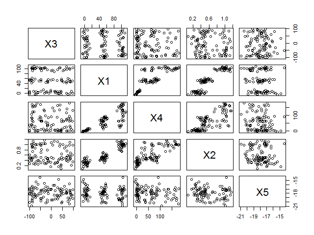
Here’s the correlation matrix and the correlogram.

cor(data)
pairs(data)

	X3	X1	X4	X2	X5
X3	1.00000000	-0.1133516	-0.08752043	-0.09320869	-0.02701275
X1	-0.11335158	1.0000000	0.83200505	0.90965123	-0.14800759
X4	-0.08752043	0.8320051	1.00000000	0.75789451	-0.15882644
X2	-0.09320869	0.9096512	0.75789451	1.00000000	-0.13261305
X5	-0.02701275	-0.1480076	-0.15882644	-0.13261305	1.00000000

Correlogram

It should already be obvious from both the correlation matrix and the correlogram that there is a strong connection between X1, X2 and X4, whereas X3 and X5 are unrelated to the rest. Let’s see whether we can confirm this with a PCA. We use the princomp function with the default parameters.

pc <- princomp(data)
summary(pc)
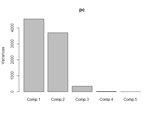
plot(pc)

Importance of components:	Comp.1	Comp.2	Comp.3	Comp.4	Comp.5
Standard deviation	67.5243440	60.8182793	18.54506263	1.2692048845	1.216295e-01
Proportion of Variance	0.5299356	0.4299031	0.03997229	0.0001872259	1.719413e-06
Cumulative Proportion	0.5299356	0.9598388	0.99981105	0.9999982806	1.000000e+00

The table shows that already component 1 and 2 together capture 96% of the data’s variance. The screeplot confirms this.

Screeplot

To find out which components match to which variables, we’ll use the loadings function.

loadings(pc)

</table>

Loadings	Comp.1	Comp.2	Comp.3	Comp.4	Comp.5
X3	0.596	0.803
X1	-0.459	0.322	0.828
X4	-0.659	0.501	-0.560
X2					1.000
X5				1.000

</tr>

	Comp.1	Comp.2	Comp.3	Comp.4	Comp.5
SS loadings	1.0	1.0	1.0	1.0	1.0
Proporation Var	0.2	0.2	0.2	0.2	0.2
Cumulative Var	0.2	0.4	0.6	0.8	1.0

Component 4 and 5 map to variables X2 and X5. They are clearly independent from the rest. Component 1, 2 and 3 map to variables X3, X1 and X4. Wait a second. Does this make sense? Something is fishy here. From how we constructed the sample dataset, we would actually expect variables X1, X2 and X4 to belong together - not X1, X3 and X4! Did we maybe make a mistake somewhere? Unfortunately we did. princomp by default uses the variance matrix - not the correlation matrix - to compute the different components. Variances unlike correlations, however, depend strongly on the scale and units of the input data. This means, either __[we must scale our input data prior to performing a principal component analysis or we must base our analysis on the correlations, not the variances, between our variables](http://stats.stackexchange.com/questions/53/pca-on-correlation-or-covariance)__. Let's quickly have a look at the variance matrix.

var(data)

	X3	X1	X4	X2	X5
X3	4043.545354	-287.916544	-307.35406	-1.74489036	-2.22236234
X1	-287.916544	1595.569658	1835.40627	10.69703439	-7.64903703
X4	-307.354064	1835.406265	3049.97811	12.32218479	-11.34843658
X2	-1.744890	10.697034	12.32218	0.08666848	-0.05051051
X5	-2.222362	-7.649037	-11.34844	-0.05051051	1.67390100

Note how very different the result looks compared to the correlation matrix above. For example (in absolute numbers) the variance between X1 and X3 is much higher than the variance between X1 and X2, although we know for sure that the relation should actually be inverse. Looking at the correlation matrix, the relations make much more sense. Fortunately, it's pretty easy to perform a PCA based on the correlation matrix by using the cor = TRUE parameter in the princomp function.

pc <- princomp(data, cor = TRUE)
summary(pc)
plot(pc)

Importance of components:	Comp.1	Comp.2	Comp.3	Comp.4	Comp.5
Standard deviation	1.649629	1.013166	0.9597193	0.50290695	0.27972026
Proportion of Variance	0.544255	0.205301	0.1842122	0.05058308	0.01564869
Cumulative Proportion	0.544255	0.749556	0.9337682	0.98435131	1.00000000

![Screeplot](/public/img/2015-05-31-screeplot2.png "Screeplot") Looking at the summary output and the screeplot, we'd probably conclude that having three components would be a good choice. Let's look at the loadings.

loadings(pc)

Loadings	Comp.1	Comp.2	Comp.3	Comp.4	Comp.5
X3		0.772	0.628
X1	-0.586			-0.201	0.779
X4	-0.551			0.801	-0.218
X2	-0.569		0.118	-0.564	-0.587
X5	0.144	-0.635	0.759

</tr> </tbody></table> This certainly looks better. X3, X1 and X2 now seem to be related together. Interestingly though X3 and X5 also seem to be related. From the loadings table alone, we would certainly still find it difficult to guess that they are actually independent from each other. However, in combination with the correlation matrix further above we could conclude that indeed X1, X2 and X4 belong together since they are highly correlated, and that furthermore X3 and X5 must be separated from each other because they are not correlated. This would then result in three components. From here we could now go on to rotate our components if we wanted to. ---- Here are a few other good tutorials on PCA: * [http://www.statmethods.net/advstats/factor.html](http://www.statmethods.net/advstats/factor.html) * [http://www.r-bloggers.com/pca-and-k-means-clustering-of-delta-aircraft/](http://www.statmethods.net/advstats/factor.html) * [http://ocw.jhsph.edu/courses/statisticspsychosocialresearch/pdfs/lecture8.pdf](http://ocw.jhsph.edu/courses/statisticspsychosocialresearch/pdfs/lecture8.pdf) From all the available videos on Youtube on this topic, I especially liked this one: This video gives a good overview on the theoretical background of the principal component analysis: Once you have performed a principal component analysis, you might then want to perform a principal component regression.

</td>	Comp.1	Comp.2	Comp.3	Comp.4	Comp.5
SS loadings	1.0	1.0	1.0	1.0	1.0
Proportion Var	0.2	0.2	0.2	0.2	0.2
Cumulative Var	0.2	0.4	0.6	0.8	1.0

Fabian Kostadinov

Principal Component Analysis in R