Cointegration and the Role of the Intercept
Yesterday I wanted to find out whether a pair of stocks would be suitable for pair trading. There is a tutorial by Paul Teetor how to test a pair of securities for cointegration. Basically, we use an OLS linear regression model to estimate the absolute prices of one security with the other’s prices. If the residuals, i.e. the spreads, are stationary then we can conclude that both time series are mean-reverting. This implies that both securities are cointegrated. However, one thing remained unclear to me after first going through Teetor’s tutorial - the role of the intercept in the regression model. In the tutorial, when estimating the regression model Teetor explicitly sets the intercept to 0 without explaining further why and what the implications are. As it happened, the two stocks I had selected are a great example to study the effect this choice has.
The following is some R code. First, I loaded the stock data using the quantmod and a few other packages. Looking at a ten years time frame is a questionable decision if the goal is to create a pairs trading strategy, but in this example I’ll do it anyway.
library(xts)
library(tseries)
library(quantmod)
library(fUnitRoots)

from.dat <- as.Date("01/06/2004", format="%d/%m/%Y")
to.dat <- as.Date("03/01/2015", format="%d/%m/%Y")

getSymbols("StockA", src="yahoo", from = from.dat, to = to.dat)
getSymbols("StockB", src="yahoo", from = from.dat, to = to.dat)

# Let's create some charts of the adjusted close series
plot.zoo(merge(Ad(StockA), Ad(StockB)), plot.type = "single", col = c("red", "blue"), xlab = "Year", ylab = "Stock Price")
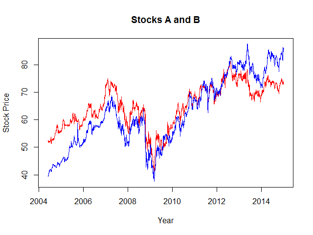
This outputs the following chart:
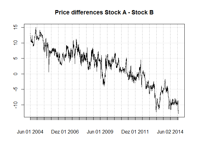
 Obviously, the stocks are correlated. Whether or not they are cointegrated remains to be decided. Interestingly, over the years the blue stock outperforms the red stock slowly but constantly. This becomes clear if we plot the price differences between the stocks.
tmp <- merge(Ad(StockA), Ad(StockB))
plot(tmp[,1] - tmp[,2], main = "Price differences Stock A - Stock B")
Let’s use a
 lm regression model to calculate the spreads. Be aware that we explicitly set the intercept to 0.
m <- lm(Ad(StockA) ~ Ad(StockB) + 0)
plot(m$residuals, main = "Residuals")

# The following is not really needed but makes the point clear
intercept <- 0
hedgeRatio <- coef(m)[1]

# sprd contains the same values as m$residuals
sprd <- Ad(StockA) - hedgeRatio * Ad(StockB) - intercept
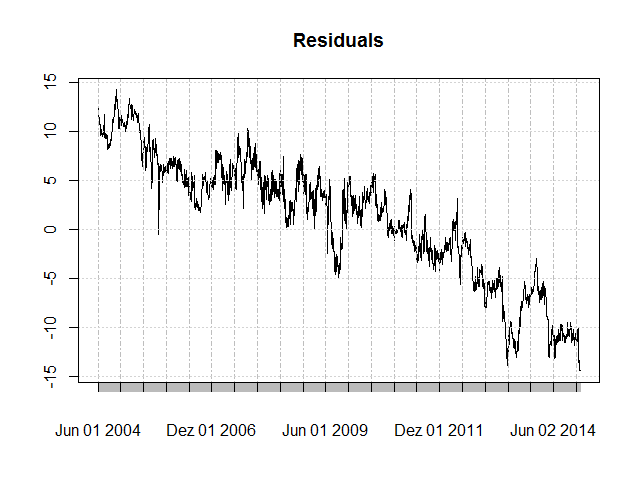
The residuals clearly show a long-term negative trend. Using stock B to estimate stock A with a zero intercept therefore systematically overestimates in the time before 2009 and systematically underestimates in the time after 2009. In fact, the residual plot seems to be the same or nearly so as the price differences plot above. Why is this so? Let’s recall what the regression formula effectively means:
Price Ai = intercept + hedgeRatio * Price Bi + Errori
We forced the intercept to be 0. Therefore, Price A is a linear combination of Price B - hence the hedgeRatio (or beta) plus an error term (the residual). The sum of the residuals is necessarily 0 in an OLS regression. Therefore, the residual plot is centered around the 0 line. Furthermore, there is only a single hedge ratio value for all observations. Stock B constantly slightly outperforms stock A over the years, and hence the residuals have the observed bias.
Let’s introduce a non-zero intercept.
m <- lm(Ad(StockA) ~ Ad(StockB))
plot(m$residuals, main = "Residuals")

# The following is not really needed but makes the point clear
intercept <- coef(m)[1]
hedgeRatio <- coef(m)[2]

# sprd contains the same values as m$residuals
sprd <- Ad(StockA) - hedgeRatio * Ad(StockB) - intercept
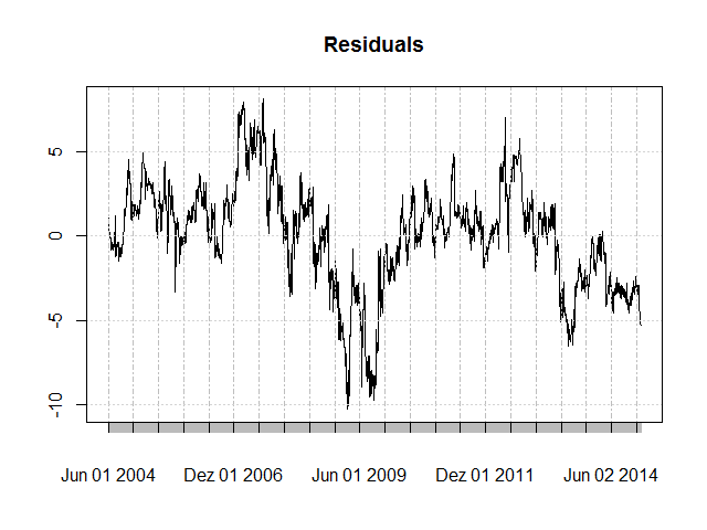
Now the residuals’ bias has disappeared. The intercept therefore “closes the gap” of the continuous outperformance of stock B over stock A, so to speak.
Let’s go on. Are the two time series cointegrated or not? We use an augmented Dickey-Fuller (ADF) test to decide. The adf.test function from the tseries package is quite handy.
adf.test(m$residuals, alternative = "stationary", k = 0)Be aware that adf.test essentially detrends your input data! This is okay for the non-zero intercept situation where our spreads are more or less without trend. Is it however also okay for the zero intercept situation where the spreads show a long-term negative trend? Well, I would say this depends on your goal. If you are implementing a short-term pair trading strategy and the spreads are trending over years, you might still be okay with a de-trended ADF test. But if your time horizon is the long-term then you cannot simply ignore the trend in the spreads. In the latter case both time series are not mean-reverting!
Here’s the output.
| Zero Intercept | Non-zero Intercept | |
|---|---|---|
| Intercept | 0 | 28.75452 |
| Hedge Ratio | 1.017733 | 0.5772449 |
| adf.test |
Augmented Dickey-Fuller Test
|
Augmented Dickey-Fuller Test
|
In both situations the Dickey-Fuller value is much lower than the 5% threshold of -2.86 (regression model without trend) or -3.41 (regression model with trend), and thus p-value < 0.05. This means that we can be more than 95% confident that the two time series are indeed cointegrated (in the short term).
Appendix
If you are not okay with the function adf.test to detrend the input data first, then there is an alternative in R. Luckily, there is another ADF test function in the fUnitRoots package called adfTest (mind the spelling). Unlike the adf.test function it lets you specify whether the underlying regression model has or has not an intercept and whether the input time series for the regression has or has not a trend. This short Youtube video explains the situation.
From the video:
When we take [the] log of any financial series, the trend of that series vanishes. So when we do ADF on log of prices then only intercept should be included [but] not trend. But if we do the ADF at level (original prices, not log) then intercept and trend should be considered at level. But for first differences only intercept should be considered.
Another good explanation can be found in this discussion thread.
Stock prices nearly always have a long-term trend, they are not stationary. Furthermore, their levels (original prices) are always different from 0, therefore an intercept is required in the ADF test.
However, remember that before we were not looking at stock prices. Instead, we were looking at residuals, i.e. spreads between two price series. If the residuals are stationary, then we know that both time series are mean-reverting, which indicates that they are cointegrated and a good candidate for a pair trading strategy. If the spreads have a clearly visible trend, then they are already guaranteed not to be stationary. Hence:
adfTest(m$residuals, lags = 0, type = "c")